Seeding Demonstration
Iris Dataset
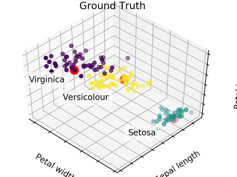
An easy way to see the quality of the seedings chosen by each of these algorithms is visualizing the seed choices on top of the frequently used “Iris” dataset in sklearn.
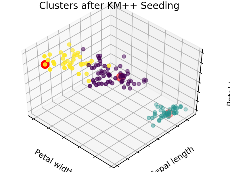
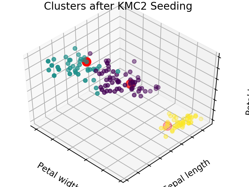
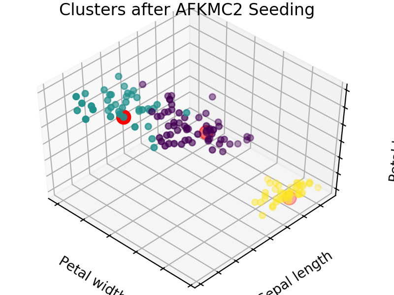

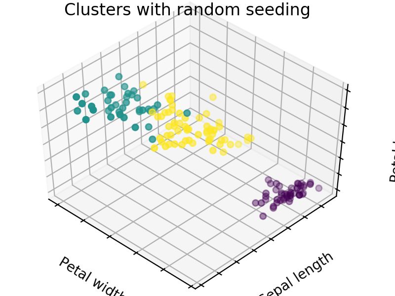
We easily see that each algorithm finds reasonable choices for seeds that barely differ from each other. These seedings allow KMeans to categorize the data well, we can see that by comparing tot he ground truth shown below. Clusters with random seedings are shown below as well, we see that KMeans still converges at a good solution since this is an easy problem, but the number of iterations needed to get there was higher.
We expect KM++ and AFKMC2 to have the highest quality seedings while KMC2 might in some cases suffer from a poor choice of assumed distribution. The main difference between KM++ and AFKMC2 will be visible when looking at runtime.
Runtime Comparison
The time complexity of using one of the KMC^2 approaches over KM++ clearly shows for larger datasets.
Average Runtime for 50 passes, 40 dimensions and 3 centers
| Size | KM++ | KMC2 | AFKMC2 | AFKMC2C |
|---|---|---|---|---|
| 200 | .0031 | .0054 | .0133 | .0107 |
| 1000 | .014 | .0053 | .0204 | .01899 |
| 5000 | .07838 | .00556 | .05683 | .058771 |
| 20000 | .29286 | .00529 | .17766 | .188594 |
| 100000 | .59260 | .0057 | .87167 | .929336 |
While on a set with 200 observations and 40 dimensions KM++ outperforms the others, the MCMC approaches bring large time savings for datasets with 2000+ observations. We can still feel the one pass over n in the AF approaches, but if the number of centers increases KM++ would feel a strong increase in runtime while AFKMC2 is barely affected as shown below.
| Size | K | Dimensions | KM++ | KMC2 | AFKMC2 | AFKMC2C |
|---|---|---|---|---|---|---|
| 100000 | 3 | 40 | .59260 | .0057 | .87167 | .929336 |
| 100000 | 6 | 40 | 6.9294 | .01998 | 1.4054 | 1.47619 |
| 100000 | 3 | 80 | 1.5638 | .00559 | .86605 | .924057 |
| 500 | 20 | 80 | .43924 | .20874 | .28856 | .173561 |
We notice that the proposed addition of caching reduces performances in situations with numbers of observations. This is due to the fact that we save between (1-k)*m and .5*(1-k)^2*m passes over the data. Since MCMC does not need to increase m for large datasets we will only save slightly above 1200 calculations for the case with 6 centers and 100000 points but still have to do at least 101000 calculations. Only the last example shows a case in which the time saving due to caching is significant and clearly outperforms all other cases since in a dataset with 500 points we are more likely to have duplicates among our 200 points in the Markov Chain.